Python绘制六种可视化图表
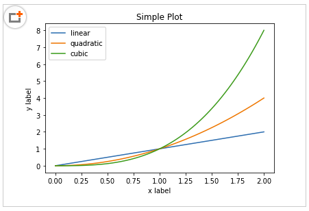
01. 折线图
绘制折线图,如果你数据不是很多的话,画出来的图将是曲折状态,但一旦你的数据集大起来,比如下面我们的示例,有100个点,所以我们用肉眼看到的将是一条平滑的曲线。
这里我绘制三条线,只要执行三次 plt.plot 就可以了。
|
1
2
3
4
5
6
7
8
9
10
11
|
importnumpy as np
importmatplotlib.pyplot as plt
x=np.linspace(0,2,100)
plt.plot(x, x, label='linear')
plt.plot(x, x**2, label='quadratic')
plt.plot(x, x**3, label='cubic')
plt.xlabel('x label')
plt.ylabel('y label')
plt.title("Simple Plot")
plt.legend()
plt.show()
|
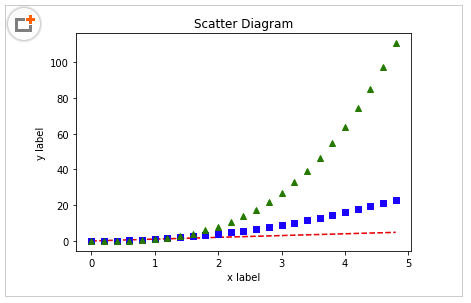
02. 散点图
其实散点图和折线图是一样的原理,将散点图里的点用线连接起来就是折线图了。所以绘制散点图,只要设置一下线型即可。
注意:这里我也绘制三条线,和上面不同的是,我只用一个 plt.plot 就可以了。
|
1
2
3
4
5
6
|
importnumpy as np
importmatplotlib.pyplot as plt
x=np.arange(0.,5.,0.2)
# 红色破折号, 蓝色方块 ,绿色三角块
plt.plot(x, x,'r--', x, x**2,'bs', x, x**3,'g^')
plt.show()
|
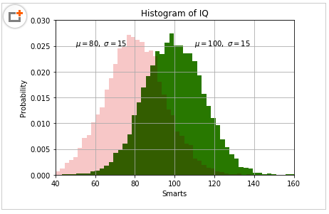
03. 直方图
直方图,大家也不算陌生了。这里小明加大难度,在一张图里,画出两个频度直方图。这应该在实际场景上也会遇到吧,因为这样真的很方便比较,有木有?
|
1
2
3
4
5
6
7
8
9
10
11
12
13
14
15
16
17
18
19
20
21
22
23
|
importnumpy as np
importmatplotlib.pyplot as plt
np.random.seed(19680801)
mu1, sigma1=100,15
mu2, sigma2=80,15
x1=mu1+sigma1*np.random.randn(10000)
x2=mu2+sigma2*np.random.randn(10000)
# the histogram of the data
# 50:将数据分成50组
# facecolor:颜色;alpha:透明度
# density:是密度而不是具体数值
n1, bins1, patches1=plt.hist(x1,50, density=True, facecolor='g', alpha=1)
n2, bins2, patches2=plt.hist(x2,50, density=True, facecolor='r', alpha=0.2)
# n:概率值;bins:具体数值;patches:直方图对象。
plt.xlabel('Smarts')
plt.ylabel('Probability')
plt.title('Histogram of IQ')
plt.text(110, .025, r'$\mu=100,\ \sigma=15$')
plt.text(50, .025, r'$\mu=80,\ \sigma=15$')
# 设置x,y轴的具体范围
plt.axis([40,160,0,0.03])
plt.grid(True)
plt.show()
|
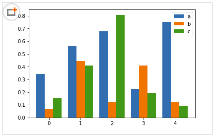
04. 柱状图
同样的,简单的柱状图,我就不画了,这里画三种比较难的图。
4.1 并列柱状图
|
1
2
3
4
5
6
7
8
9
10
11
12
13
14
15
16
17
18
|
importnumpy as np
importmatplotlib.pyplot as plt
size=5
a=np.random.random(size)
b=np.random.random(size)
c=np.random.random(size)
x=np.arange(size)
# 有多少个类型,只需更改n即可
total_width, n=0.8,3
width=total_width/n
# 重新拟定x的坐标
x=x-(total_width-width)/2
# 这里使用的是偏移
plt.bar(x, a, width=width, label='a')
plt.bar(x+width, b, width=width, label='b')
plt.bar(x+2*width, c, width=width, label='c')
plt.legend()
plt.show()
|
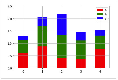
4.2 叠加柱状图
|
1
2
3
4
5
6
7
8
9
10
11
12
13
14
15
|
importnumpy as np
importmatplotlib.pyplot as plt
size=5
a=np.random.random(size)
b=np.random.random(size)
c=np.random.random(size)
x=np.arange(size)
# 这里使用的是偏移
plt.bar(x, a, width=0.5, label='a',fc='r')
plt.bar(x, b, bottom=a, width=0.5, label='b', fc='g')
plt.bar(x, c, bottom=a+b, width=0.5, label='c', fc='b')
plt.ylim(0,2.5)
plt.legend()
plt.grid(True)
plt.show()
|
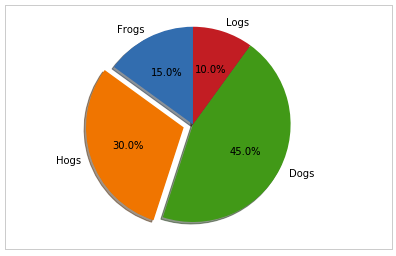
05. 饼图
5.1 普通饼图
|
1
2
3
4
5
6
7
8
9
10
|
importmatplotlib.pyplot as plt
labels='Frogs','Hogs','Dogs','Logs'
sizes=[15,30,45,10]
# 设置分离的距离,0表示不分离
explode=(0,0.1,0,0)
plt.pie(sizes, explode=explode, labels=labels, autopct='%1.1f%%',
shadow=True, startangle=90)
# Equal aspect ratio 保证画出的图是正圆形
plt.axis('equal')
plt.show()
|
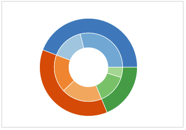
5.2 嵌套饼图
|
1
2
3
4
5
6
7
8
9
10
11
12
13
14
15
16
17
18
19
20
|
importnumpy as np
importmatplotlib.pyplot as plt
# 设置每环的宽度
size=0.3
vals=np.array([[60.,32.], [37.,40.], [29.,10.]])
# 通过get_cmap随机获取颜色
cmap=plt.get_cmap("tab20c")
outer_colors=cmap(np.arange(3)*4)
inner_colors=cmap(np.array([1,2,5,6,9,10]))
print(vals.sum(axis=1))
# [92. 77. 39.]
plt.pie(vals.sum(axis=1), radius=1, colors=outer_colors,
wedgeprops=dict(width=size, edgecolor='w'))
print(vals.flatten())
# [60. 32. 37. 40. 29. 10.]
plt.pie(vals.flatten(), radius=1-size, colors=inner_colors,
wedgeprops=dict(width=size, edgecolor='w'))
# equal 使得为正圆
plt.axis('equal')
plt.show()
|
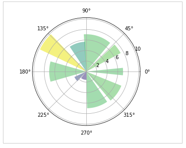
5.3 极轴饼图
要说酷炫,极轴饼图也是数一数二的了,这里肯定也要学一下。
|
1
2
3
4
5
6
7
8
9
10
11
12
13
14
15
16
17
|
importnumpy as np
importmatplotlib.pyplot as plt
np.random.seed(19680801)
N=10
theta=np.linspace(0.0,2*np.pi, N, endpoint=False)
radii=10*np.random.rand(N)
width=np.pi/4*np.random.rand(N)
ax=plt.subplot(111, projection='polar')
bars=ax.bar(theta, radii, width=width, bottom=0.0)
# left表示从哪开始,
# radii表示从中心点向边缘绘制的长度(半径)
# width表示末端的弧长
# 自定义颜色和不透明度
forr, barinzip(radii, bars):
bar.set_facecolor(plt.cm.viridis(r/10.))
bar.set_alpha(0.5)
plt.show()
|
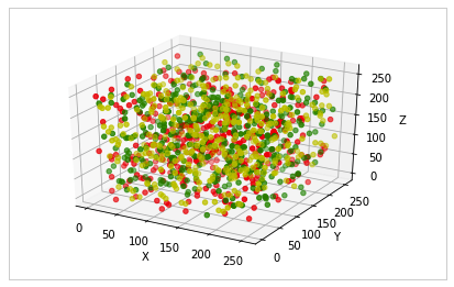
06. 三维图
6.1 绘制三维散点图
|
1
2
3
4
5
6
7
8
9
10
11
12
13
14
|
importnumpy as np
importmatplotlib.pyplot as plt
frommpl_toolkits.mplot3dimportAxes3D
data=np.random.randint(0,255, size=[40,40,40])
x, y, z=data[0], data[1], data[2]
ax=plt.subplot(111, projection='3d')# 创建一个三维的绘图工程
# 将数据点分成三部分画,在颜色上有区分度
ax.scatter(x[:10], y[:10], z[:10], c='y')# 绘制数据点
ax.scatter(x[10:20], y[10:20], z[10:20], c='r')
ax.scatter(x[30:40], y[30:40], z[30:40], c='g')
ax.set_zlabel('Z')# 坐标轴
ax.set_ylabel('Y')
ax.set_xlabel('X')
plt.show()
|
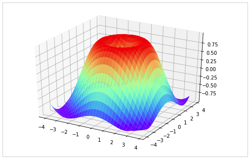
6.2 绘制三维平面图
|
1
2
3
4
5
6
7
8
9
10
11
12
13
|
frommatplotlibimportpyplot as plt
importnumpy as np
frommpl_toolkits.mplot3dimportAxes3D
fig=plt.figure()
ax=Axes3D(fig)
X=np.arange(-4,4,0.25)
Y=np.arange(-4,4,0.25)
X, Y=np.meshgrid(X, Y)
R=np.sqrt(X**2+Y**2)
Z=np.sin(R)
# 具体函数方法可用 help(function) 查看,如:help(ax.plot_surface)
ax.plot_surface(X, Y, Z, rstride=1, cstride=1, cmap='rainbow')
plt.show()
|
总结
以上所述是小编给大家介绍的Python绘制六种可视化图表,希望对大家有所帮助,如果大家有任何疑问请给我留言,小编会及时回复大家的。在此也非常感谢大家对脚本之家网站的支持!